Github webpage : https://pauloacs.github.io/Deep-Learning-for-solving-the-poisson-equation/
The approaches can be mainly classified by the way the simulation data is treated. In I the data (in this case 2D unsteady simulations): each frame of the simulation is used as an image to use typical convolutional models.
To overcome the drawbacks of the above method, and be able to take data from any mesh without interpolation to a uniform grid (resembling pixels of an image) and without losing information in zones of particular interest in the further methods, in II, III, IV the data extracted as points of a domain (representing the cells of a mesh - including those at the boundaries).
Backward_facing step simulations and model as in: https://github.com/IllusoryTime/Image-Based-CFD-Using-Deep-Learning.
Inspired in the mentioned repository the unsteady nature of the Kármán vortex street is predicted. The process of voxelization and the model were symilar to similar to the above mentioned work.
...explain how the voxelization is done...
No info is given about the geometry, either way, the model can learn. IMPORTANT NOTE: In this method, the features (physical quantities) are mapped directly and that process may be influenced by the order in which the points are given therefore making the model not able to generalize to a differently organized set of points of the same flow. To achieve invariance in this aspect, proceed to section II.
** Esquema da rede **
The model takes all the previous known values and based on those, predicts the value for the next time.
(sims, times, points, feature) --> (sims, times, points, feature)
Training with all the timesteps, but the goal is to use it with n previous know times, for example:
(sim, 1, ...) ---predict---> (sim, 2, ...)
(sim, 1&2, ...) ---predict---> (sim, 2&3, ...)
(sim, 1&2&3, ...) ---predict---> (sim, 2&3&4, ...) ...and so on...
Problem: Loss becomes nan - solved: Do not use "relu" activation in LSTM - it leads to exploding gradients (can also be solved with clipvalue in the adam optimizer but it harms the training(a lot))
- 1 780 000 parameters
** Esquema da rede **
This model predicts only the next time value of a field, having as input the field at the present time.
(sims * times , points, feature) --> (sims * times, points, feature)
The best test loss archived so far ~ 2e-3.
Defining the loss as:
As expected this architecture has troubles in generalization. Should process to work only with the ones with coordinate information. This models mimic the ones with image data, but convolutions in image data have information about location and here they don't.
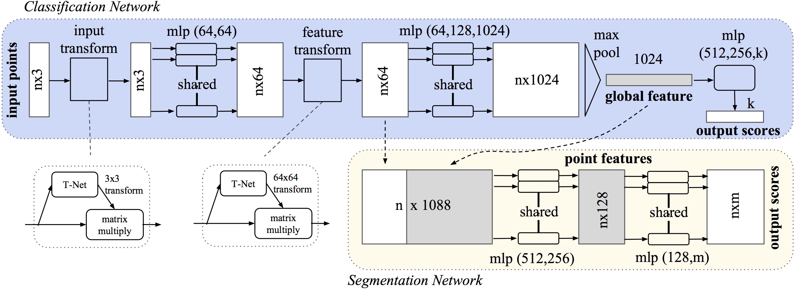
PointNet (https://github.com/charlesq34/pointnet) concept is joined with the networks presented in the last section giving information about the geometry (x and y values). For getting the spatial coordinates of each cell center the OpenFOAM's post-processing utility - writeCellCentres - is used. The original PointNet architecture is presented in the following image, the segmentation network is the one of interest in this case.
PointNet is successfully used to predict flow quantities in https://arxiv.org/abs/2010.09469 for stationary flows, hence only giving coordinate information. Here the ultimate goal is to tackle the unsteady evolution of a flow.
The networks here developed will be introduced now:
** Esquema da rede **
- 2 560 000 parameters
** Esquema da rede **
- 2 670 000 parameters
Since the ultimate goal is to, from the previous velocity field, predict the pressure and it needs to be done for every cell of the mesh, the training of the model was done with all cells.
CONV+PointNet : 50 epoch training with 100 simulations in the training set. (with padding and not ignoring the padded values)

Using every cell for training revealed itself too expensive so now I'm using only 1/4 of the data. Maybe it can be trained with N cells: input:(...,N) --> output(...,N) but be able to do: input:(...,other_N) --> output(...,other_N) with other_N > N. Try this
.gif) ** Representar os resultados reais e não os normalizados na próxima atualização, faltou "desnormalizar" **
** Representar os resultados reais e não os normalizados na próxima atualização, faltou "desnormalizar" **
Stop trying to predict from the 0-th time. The evolution from the initial conditions to the first time is very different from the evolution between times. As can be seen in the shown predictions, the model can not, with so little data, learn to predict that.
TRAIN TO PREDICT THE STREAM FUNCTION IN THE PREVIOUS MODELS - WILL ENFORCE CONTINUITY - THE DRAWBACK - ONLY WORKS FOR 2D
Using OpenFOAM's postprocessing utility by typing :
postprocess -func streamfunction
Now modifying the above models to predict instead of the velocity vector, it will ensure continuity.
Since streamFunction is a PointScalarField and we are using the vaues at the cell centers - volScalarField, it need to be interpolated:
directly in openfoam it could be done by creating a volScalarField: streamFunction_vol and using the following function:
pointVolInterpolation::interpolate(streamFunction);
Another option is to interpolate in python, for this griddata from scipy.interpolate is used.
To refine the understanding and implement one of these networks, firstly (as it is common in literature), the implementation of a model which can predict the flow given the boundary, initial conditions and governing equations is implemented. It needs no data from the CFD solver since it only needs to be given the coordinates of a sample of points and the parameters at the initial time.
The governing equations are not evaluated in every point, instead, a random sample of the points' coordinates is taken and the residuals are calculated for those. Random sample first - cheaper. Use Latin hypercube sampling (lhs) sampling later: https://idaes-pse.readthedocs.io/en/1.5.1/surrogate/pysmo/pysmo_lhs.html. lhs sampling from idaes has two modes: sampling and generation.
In the more common examples in literature, the generation mode is chosen, it is much faster than the sampling one but here the purpose is to use a grid previously defined in OpenFOAM - allowing applicability to the correction model which will be definied ahead and automatization since scripts to generate meshes are already programmed and are present in the data folder. LHS sampling in the sampling mode is very computational expensive, therefore at this point ramdom sampling is employed in detriment of lhs.
lhs in generation mode could be used but it would not generalize to complex shapes since the procedure is to generate points within a rectangle and only after exclude those inside the obstacle. (unless I export points from all the boundaries and write a function which deletes points inside/outside of them.
B - Boundaries and GE - Governing equations IC - Initial conditions
with:
- Does not converge yet. Needs 2nd order derivations. The advantage is that this models is not constraint to 2D problems, making it work would be helpful.
Ux and Uy are derived from :
The stream function enforces continuity since:
For steady-state flow the following results were archieved:

The training consisted in:
- 10000 Adam optimization iterations
- 50000 L-BFGS iterations Showing a very good prediction from the PINN.
For transient flow the loss function is defined as:
B - Boundaries and GE - Governing equations IC - Initial conditions
with:
- Leads to convergence. Needs 3rd order derivations!
The Cauchy momentum equations are used here:
with the constitutive equation for incompressible newtonian fluid:
- Leads to convergence. Needs only 2nd order derivations while ensuring continuity which makes the optimization problem easier. Higher-order derivations lead to much higher computational and storage costs.
Concept from: https://arxiv.org/abs/2002.10558
For steady-state flow the following results were archieved:

The training consisted in:
- 10000 Adam optimization iterations
- 30000 L-BFGS iterations
Showing also a good solution for the steady-state flow.
For unsteady:
B - Boundaries and GE - Governing equations IC - Initial conditions
Const being the constitutive equation.
Steady-state flow prediction is easily done:
concepts i) and ii) are implemented in their own repositories ( i) https://github.com/maziarraissi/PINNs ii) https://github.com/Raocp/PINN-laminar-flow ) in a similar code using version 1.x of tensorflow and solve the problem with a mesh generated in python (using lhs sampling).
In this repository those concepts are developed in version 2.x making use of some of its utilities but also programming a costum training loop in order to provide extra flexibility allowing to make use of complex custom functions.
This would be the model with the lowest computations cost on differentiation because only first order derivatives are needed. This could compensate the harder convergence. -did not converge yet-
NOTE THAT CONVERGENCE IN THIS MODELS IS HIGHLY DEPENDENT ON THE DEFINITION OF THE LOSS FUNCTION.
Since the models have too many parameters, differentiate multiple times, each batch in each epoch becomes prohibitively expensive (and very RAM demanding, crashing the google Colab when using 12,7 GB of RAM). To overcome this, multiple methods are being studied:
1 - using a different neural network to refine the result of one of the previous models minimizing the residuals of the governing equations and matching the boundary conditions
- not knowing the true values for the values in the interior of the domain. Using adam optimization but also L-BFGS as in https://github.com/maziarraissi/PINNs .
The loss is defined as:
B - Boundaries and GE - Governing equations IC - Initial conditions
The input coordinates are normalized as :
Ideas:
i- Coordinates as inputs (3 input features) and parameters as outputs having the parameters predicted by the "Convmodel" helping in the training.
ii - Coordinates and parameters predicted by the "ConvModel" as inputs (6 input features) - fast to approach the loss of the ConvModel but can overfit in a way hard to overcome.

The layers connecting to the left side of the "add layer" can be thought of as providing an offset to the results provided on the right-hand side.
version 2:
.jpg)
2 - retrain the big model (update its parameters) for only one prediction with the loss as defined above.
To do: Test "adaptive activation functions" to speed up training. (https://www.researchgate.net/publication/337511438_Adaptive_activation_functions_accelerate_convergence_in_deep_and_physics-informed_neural_networks)
- PointNET++: https://arxiv.org/abs/1706.02413
- PointConv: https://arxiv.org/abs/1811.07246
- SO-NET: https://arxiv.org/abs/1803.04249
- PSTNET: https://openreview.net/pdf?id=O3bqkf_Puys
The Navier-Stokes equations for incompressible flow are (neglecting the gravity term):
and can be non-dimensionalized to:
with
U is the mean velocity (a parabolic profile is implemented at the inlet) fixed at 1. H = 1 , nu = 5e-3 Re= 200 (<1400 for laminar flow between parallel plates)
1st simulation: squared cylinder
2nd : squared cylinder + cylinder + elipses
To increase training performance, the data was further normalized to be in [0-1] range making the pressure (typical bigger value) having the same relevance as the velocity.
where is some physical quantity. The max and min values are those of the whole training set.
As all the simulations do not have the same number of cells, when exporting the data, the data was padded, and since convolutional models do not allow masking, in the loss function the padded values are not accounted for.