Contents

• Neural Networks => nn.ipynb
  • Logistic Regression
  • MLP
    • Forward Propagation (Explained on Pen and Paper)
    • Back Propagation (Equations Derived on Pen and Paper)
    • Gradient Descent
    • Train Loop
    • Results
• Batch-Normalization and Layer-Normalization: Why When Where & How? => batchnorm.ipynb, layernorm.ipynb
  • Batch-Normalization
  • Layer-Normalization
  • Comparision
• Dropout: Why When Where & How? => dropout.ipynb, dropout_scale.ipynb
  • Comparision before and after scaling the model => dropout_scale.ipynb, nn_scale.ipynb
• Adam and AdamW
  • Adam
  • AdamW
• Model Distillation => distillation.ipynb
• Mixture-Of-Experts (MoE) Layers

Neural Networks

Aim of this repo

• This repo aims to make you an MLPWhiz (especially a BackpropWhiz) by creating a Neural Network from scratch just using torch.tensor (NO using torch's autograd) and training them on the MNIST dataset (A dataset containing handwritten digits from 0 to 9)

Roadmap

• The best way to go about this tutorial is to take a pencil and a piece of paper and start deriving particularly the backprop equations once you get the concept
• First we'll start off with logistic regression, which is the simpler form of MLPs just containing 1 layer and can recognize 2 classes, then scale into MLPs by adding many layers and making it recognize as many classes as you want

Logistic Regression

• Now suppose we want to build a model that classifies a handwritten digit 9 vs any digit that is not 9

• The input to the model are the pixels of the image (which are the features) which are to be linearly transformed so that they can classify the digits, this is done with the help of learnable parameters learned from the data that we will provide

• And here we have to classify 9 vs not 9 so we only need one unit in the last layer (in MLPs we have many classes so we have n_classes number of units in the last layer where n_classes is the number of classes which will represent the probabilities for the n_classes given input)

• Sigmoid function:

  This function squishes the pre-activations (Z) to have a range of (0, 1)

• Then we define a threshold (which is usually 0.5), if the probabilities are above it then the digit is 9 else it's not

• Take a look at the below example
  

• Forwardprop

  X = inputs.reshape((B, H*W*1)) # (B, F=H*W) <= (B, H, W, 1) = (Batch, Height, Width, Num_Channels)
  """
  X = [
       [x00, x01, ..., x0W,
        x10, x11, ..., x1W,
        ...
        xH0, xH1, ..., xHW],
        ... (more batches of examples)
      ]
  """
  W = [[w00], # (F, 1)
       [w10],
       ...
       [wF0]]
  B = [[b0]] # (1, 1) # broadcasted and added to element in Z
  Z = X @ W + B # (B, 1) <= (B, F) @ (F, 1) + (1, 1)
  """
  Z = [[z1 = x00*w00 + x01*w10 + ... + xHW*wF0 + b0],
      ... (more batches of examples)
      ]
  """
  A = sigmoid(Z) # (B, 1)

• Z contains Unnormalized probabilities, the sigmoid function normalizes (range: 0-1) Z to get probabilities of whether the digit is 9 (the higher the probability, the more confident the model is that the digit is 9)

• Cost function: We have to penalize the model for predicting wrong values and reward it for predicting the right values

  We want to minimize the loss to improve our model

  Therefore we use the loss function: which just means that if

  y_i = 1 (digit is 9); Loss is -log(a_i) which is negative log-probability of the digit is 9; So we want to minimize -log(a_i) which means we want to maximize a_i (the probability of digit being 9) when the digit is actually 9 which is what we want

  y_i = 0 (digit is not 9); Loss is -log(1 - a_i) which is negative log-probability of the digit not being 9; So we want to minimize -log(1 - a_i) which means we want to maximize 1 - a_i (the probability of digit not being 9) when the digit is not 9 which is again what we want

• Now using the below equations, we'll calculate how we should change the parameters so that they incorporate the learnings from the cost function and make the model better
  
  where Y is the true classes (9 or not 9)
  We'll go through the derivations for the gradients in detail in the MLPs section below

• We'll change the parameters according to the equations below
  W = W - lr * dJ_dW
B = B - lr * dJ_dB
  

• The above processes are usually not done taking the whole training set, this results in accurate gradients but this process is very slow as in deep learning, datasets are very large
  Instead we take batch_size number of train examples from the dataset and do the above process, this results in the gradients being less accurate but this is much faster and has proved to be very much effective in practice

• We repeat the above processes for a number of epochs, till the model converges, see the training loop sub-section in the MLPs section for more details

---

MLPs

Forward Propagation

• We stack many layers with a relu activation in-between layers and at the end add a softmax layer which calculates the probabilities given unnormalized activations
• Here unlike the sigmoid function we have n_classes number of units in the last layer where n_classes is the number of classes where each unit will represent the probabilities for each class given input
• 
• Cross Entropy Loss calculation: We want to increase the probabilities of the true classes, therefore we minimize negative log-probs which does the same

Back-propagation

• 
• 
• 
• 
• 
• 

Gradient Descent

• The negative gradient tells us the direction that corresponds to the steepest descent within an infinitesimally small region surrounding the current parameters
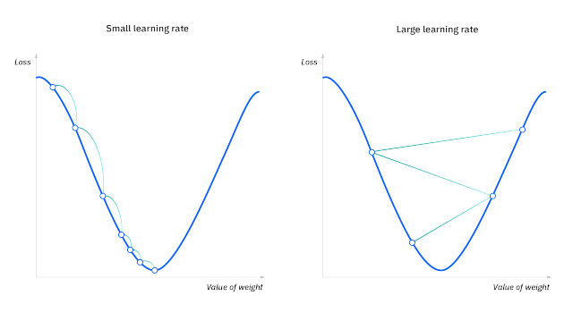
• So it's important to scale them down so that the training is stable, we do this with the help of the learning rate (lr), always keeping it less than 1 ( for very deep models we keep the lr of the order 1e-3 to 1e-5 so that the training is stable)
• We want to minimize the Loss (with the weights and biases as the parameters), we want to go down to the lowest point, the negative gradients give us the direction to the lowest point, and subtracting the parameters from their scaled-down gradients takes us downhill the Loss landscape
  

• params = [w1, b1, w2, b2, w3, b3]
  grads = [dL_dw1, dL_db1, dL_dw2, dL_db2, dL_dw3, dL_db3]
  
  for i in range(len(params)):
      params[i] = params[i] - lr*grads[i]

• Additional Note: Neural Network optimization is a non-convex optimization problem
  

---

Training Loop

• for epoch in range(epochs):
      for step in range(steps):
          X_batch, y_batch = get_batch(X, y)
          # forward prop
          # backward prop
          # gradient descent
          ...

  In one step the model is trained on batch_size number of train examples
  In one epoch which contains steps number of steps, the model is trained on all the train examples
  This done for epochs number of epochs, till the model converges

---

Results

Train Accuracy:      0.9969 | Train Loss: 0.0187 |
Validation Accuracy: 0.9794 | Validation Loss: 0.0665 |

• See the notebook to see predictions

Batch-Normalization and Layer-Normalization

Batch-Normalization

• 
• Training Deep Neural Networks is complicated by the fact that the distribution of each layer's inputs changes during training, as the parameters of the previous layers change.
• This slows down the training by requiring lower learning rates and careful parameter initialization, and makes it notoriously hard to train models with saturating nonlinearities.
• We refer to this phenomenon as internal covariate shift, and address the problem by normalizing layer inputs
• Our methoddraws its strength from making normalization a part of the modelarchitecture and performingthe normalization for each training mini-batch
• Batch Normalization allows us to use much higher learningrates and be less careful about initialization
• Batch Normalization achieves the same accuracy with 14 times fewer training steps, and beats the original model by a significant margin
• The change in the distributions of layers' inputs presents a problem because the layers need to continuously adapt to the new distribution. When the input distribution to a learning system changes, it is said to experience covariate shift
• 
• 

Layer-Normalization

• It is common among the NLP tasks to have different sentence lengths for different training cases. This is easy to deal with in an RNN because the same weights are used at every time-step. But when we apply batch normalization to an RNN in the obvious way, we need to to compute and store separate statistics for each time step in a sequence. This is problematic if a test sequence is longer than any of the training sequences. Layer normalization does not have such problem because its normalization terms depend only on the summed inputs to a layer at the current time-step. It also has only one set of gain and bias parameters shared over all time-steps.
• Here we just take mean-variance stats along the feature dimention, now no need for storing running mean and variance for inference!
• 

Comparision

• As you can see with normalization, the model learns/overfits faster than the model without normalization

• 

  No Normalization: Epoch: 30/30 | Loss: 0.0205 | Avg time per step: 0.44 ms | Validation Loss: 0.0649 |
  Batch-Normalization: Epoch: 9/30 | Loss: 0.0167 | Avg time per step: 0.79 ms | Validation Loss: 0.0899 |
  Layer-Normalization: Epoch: 14/30 | Loss: 0.0050 | Avg time per step: 0.73 ms | Validation Loss: 0.0772 |

• For some reason Validation Loss for model with normalization is not better than the model without any normalization, maybe it'll be better when the model gets deeper (i.e when number of layers increases) (correct???)

Dropout [Paper] [Deep-Learning Book]

• 

• To a first approximation, dropout can be thought of as a method of making bagging practical for ensembles of very many large neural networks

• Dropout training is not quite the same as bagging training. In the case ofbagging, the models are all independent. In the case of dropout, the modelsshare parameters, with each model inheriting a different subset of parametersfrom the parent neural network

• If a unit is retained with probability p during training, the outgoing weights of that unit are multiplied by p at test time as shown in Figure 2. This ensures that for any hidden unit the expected output (under the distribution used to drop units at training time) is the same as the actual output at test time

• In the case of bagging, each model i produces a probability distribution Because this sum includes an exponential number of terms, it is intractable to evaluate. Even 10–20 masks are often sufficient to obtaingood performance.

• An even better approach, however, allows us to obtain a good approximation tothe predictions of the entire ensemble, at the cost of only one forward propagation. To do so, we change to using the geometric mean rather than the arithmetic mean ofthe ensemble members’ predicted distributions

• 

• For many classes of models that do not have nonlinear hidden units, the weight scaling inference rule is exact

• Using Properties of exponents ($e^a*e^b = e^{a+b}$ and $\sqrt{e}=e^{1/2}$) we get Now the term in the exp (don't take the bias) is the expectation of

  which is because expectation of $d$ is just the probablity of inclusion

  

• Another method is where we would leave the inputs unchanged at inference time, but at training time we scale the retained inputs by $1/p$ where $p$ is the probabilty of inclusion. This is the method which is used in the implementation

• Dropping out 20% of the input units and 50% of the hidden units was often found to be optimal (In the simplest case, each unit is retained with a fixed probability p independent of other units, where p can be chosen using a validation set or can simply be set at 0.5, which seems to be close to optimal for a wide range of networks and tasks. For the input units, however, the optimal probability of retention is usually closer to 1 than to 0.5.)

• Bernoulli Distribution is used to mask the input values

Comparision

• Without Scaling Model
  
• After Scaling Model
  
  • In nn_scale.ipynb validation loss starts increasing... Now see dropput_scale.ipynb, the gap between training and validation metrics is lesser than in nn_scale.ipynb
  • Validation metrics has improved but at the cost of training metrics
• See the notebooks for the train logs

Adam and AdamW (Adam with weight decay) Optimizers

Adam

• 

AdamW

• What's weight decay?
  
• Paper Implementaion
• L2 regularization and weight decay regularization are equivalent for standard stochastic gradient descent (when rescaled by the learning rate), but as we demonstrate this is not the case for adaptive gradient algorithms, such as Adam
• Common implementations of these algorithms employ L2 regularization (often calling it “weight decay” in what may be misleading due to the inequivalence we expose). For example see the pytorch implementation of Adam (which is wrong) below
• $L = CE + \left(\frac{\lambda}{2}\theta^2\right)$
  $\nabla L = \nabla CE + \nabla \left(\frac{\lambda}{2}\theta^2\right) = \nabla CE + \lambda\theta$
  This is the same expression in above images/image for weight decay but it's actually for L2 Loss as shown in the equations here The corrected version is given below

Model Distillation [Paper] [Reference]

Paper Snippets

• We achieve some surprising results on MNIST and we show that we can significantly improve the acoustic model of a heavily used commercial system by distilling the knowledge in an ensemble of models into a single model
• Once the cumbersome model has been trained, we can then use a different kind of training, which we call “distillation” to transfer the knowledge from the cumbersome model to a small model that is more suitable for deployment
• When we are distilling the knowledge from a large model into a small one, however, we can train the small model to generalize in the same way as the large model
• If the cumbersome model generalizes well because, for example, it is the average of a large ensemble of differentmodels, a small model trained to generalize in the same way will typically do much better on test data than a small model that is trained in the normal way on the same training set as was used to train the ensemble.
• Use the class probabilities produced by the cumbersome model as “soft targets” for training the small model
• Probabilities are so close to zero. Caruana and his collaborators circumvent this problem by using the logits (the inputs to the final softmax) rather than the probabilities produced by the softmax as the targets for learning the small model and they minimize the squared difference between the logits produced by the cumbersome model and the logits produced by the small model
• Our more general solution, called “distillation”, is to raise the temperature of the final softmax until the cumbersome model produces a suitably soft set of targets. We then use the same high temperature when training the small model to match these soft targets. We show later that matching the logits of the cumbersome model is actually a special case of distillation.
• The transfer set that is used to train the small model could consist entirely of unlabeled data or we could use the original training set. We have found that using the original training set works well, especially if we add a small term to the objective function that encourages the small model to predict the true targets as well as matching the soft targets provided by the cumbersome model.

Distillation

• 

Preliminary experiments on MNIST

• We trained a single large neural net with two hidden layers of 1200 rectified linear hidden units on all 60,000 training cases
• The net was strongly regularized using dropout and weight-constraints as described in [5]. Dropout can be viewed as a way of training an exponentially large ensemble of models that share weights
• In addition, the input images were jittered by up to two pixels in any direction
• This net achieved 67 test errors whereas a smaller net with two hidden layers of 800 rectified linear hidden units and no regularization achieved 146 errors. But if the smaller net was regularized solely by adding the additional task of matching the soft targets produced by the large net at a temperature of 20, it achieved 74 test errors. This shows that soft targets can transfer a great deal of knowledge to the distilled model, including the knowledge about how to generalize that is learned from translated training data even though the transfer set does not contain any translations
• When the distilled net had 300 or more units in each of its two hidden layers, all temperatures above 8 gave fairly similar results. But when this was radically reduced to 30 units per layer, temperatures in the range 2.5 to 4 worked significantly better than higher or lower temperatures
• We then tried omitting all examples of the digit 3 from the transfer set. So from the perspective of the distilled model, 3 is a mythical digit that it has never seen. Despite this, the distilled model only makes 206 test errors of which 133 are on the 1010 threes in the test set. Most of the errors are caused by the fact that the learned bias for the 3 class is much too low. If this bias is increased by 3.5 (which optimizes overall performance on the test set), the distilled model makes 109 errors of which 14 are on 3s. So with the right bias, the distilled model gets 98.6% of the test 3s correct despite never having seen a 3 during training. If the transfer set contains only the 7s and 8s from the training set, the distilled model makes 47.3% test errors, but when the biases for 7 and 8 are reduced by 7.6 to optimize test performance, this falls to 13.2% test errors

model.fc.bias.data[3] += 3.5

Soft-Targets as Regularizers

• One of our main claims about using soft targets instead of hard targets is that a lot of helpful infor nation can be carried in soft targets that could not possibly be encoded with a single hard target.

Mixture-of-Experts (MoE) layer

• The capacity of a neural network to absorb information is limited by its number of parameters. Conditional computation, where parts of the network are active on a per-example basis, has been proposed in theory as a way of dramatically increasing model capacity without a proportional increase in computation. there are significant algorithmic and performance challenges
• In this work, we address these challenges and finally realize the promise of conditional computation, achieving greater than 1000x improvements in model capacity with only minor losses in computational efficiency on modern GPU clusters.
• We introduce a Sparsely-Gated Mixture-of-Experts layer (MoE), consisting of up to thousands of feed-forward sub-networks. A trainable gating network determines a sparse combination of these experts to use for each example

Introduction

• For typical deep learning models, where the entire model is activated for every example, this leads to a roughly quadratic blow-up in training costs, as both the model size and the number of training examples increase
• Various forms of conditional computation have been proposed as a way to increase model capacity without a proportional increase in computational costs, in these schemes, large parts of a network are active or inactive on a per-example basis. The gating decisions may be binary or sparse and continuous, stochastic or deterministic. Various forms of reinforcement learning and back-propagation are proposed for trarining the gating decisions

THE SPARSELY-GATED MIXTURE-OF-EXPERTS LAYER

• 
• A Sparsely-Gated Mixture-of-Experts Layer (MoE). The MoE consists of a number of experts, each a simple feed-forward neural network, and a trainable gating network which selects a sparse combination of the experts to process each input (see Figure 1). All parts of the network are trained jointly by back-propagation
• 

In MoE, whenever the gated value function returns 0, we need not compute that particular function, but it's parameters are in memory, so we are saving computation power not memory

Gating Network

• 
• 

ADDRESSING PERFORMANCE CHALLENGES

• If the gating network chooses $k$ out of $n$ experts for each example, then for a batch of $b$ examples, each expert receives a much smaller batch of approximately $kb/n << b$ examples. This causes a naive MoE implementation to become very inefficient as the number of experts increases. The solution to this shrinking batch problem is to make the original batch size as large as possible. However, batch size tends to be limited by the memory necessary to store activations between the forwards and backwards passes. We propose the following techniques for increasing the batch size:
  • (i) Mixing Data Parallelism and Model Parallelism: In the case of a hierarchical MoE (Section B), the primary gating network employs data parallelism, and the secondary MoEs employ model parallelism. Each secondary MoE resides on one device
  • (ii) Taking Advantage of Convolutionality: In our language models (RNNs not Transformers (invented later in late 2017)), we apply the same MoE to each time step of the previous layer. If we wait for the previous layer to finish, we can apply the MoE to all the time steps together as one big batch. Doing so increases the size of the input batch to the MoE layer by a factor of the number of unrolled time steps
  • (iii) Increasing Batch Size for a Recurrent MoE: We suspect that even more powerful models may involve applying a MoE recurrently. For example, the weight matrices of a LSTM or other RNN could be replaced by a MoE. Sadly, such models break the convolutional trick from the last paragraph, since the input to the MoE at one timestep depends on the output of the MoE at the previous timestep. Gruslys et al. (2016) describe a technique for drastically reducing the number of stored activations in an unrolled RNN, at the cost of recomputing forward activations. This would allow for a large increase in batch size

Balancing Expert Utilization

• 
• 
• 
  $Load(x)$ => Probability of Selection $P(x, i)$: $G(x)$ is nonzero for expert $i$ if and only if the gating score $H(x)_i$ (raw gating output before thresholding) is greater than the $k^{\text{th}}$ -greatest score among all other experts
• $Φ$ is the CDF (Gaussian cumulative distribution function) of the standard normal distribution
• Let's break down the Load Balancing Loss: we have to minimize $L_{load} (X)$, so we have to minimize $CV(Load(X))$, hence, we have to reduce the standard deviation of Load, which means most values are centred around the mean, forcing most values to be near the mean, same for $L_{importance}$

---

Contribution guidelines

• This repository aims to demystify neural networks, and any efforts aimed at simplification and enhancing accessibility will be incorporated
• Contributions towards changing the handwritten equations into LaTeX format are welcomed and encouraged.

---

References

• Blog: Sigmoid, Softmax and their derivatives
• Video: Becoming a Backprop Ninja
• Batch-Norm, Layer-Norm, Dropout, Adam and AdamW Papers

For Further Studies

• Video: Neural Networks: Zero to Hero
• Book: Deep Learning by Ian Goodfellow

---

Karpathy's blog "A Recipe for Training Neural Networks" snippets

• I have developed a specific process for myself that I follow when applying a neural net to a new problem, which I will try to describe. You will see that it takes the two principles above very seriously. In particular, it builds from simple to complex and at every step of the way we make concrete hypotheses about what will happen and then either validate them with an experiment or investigate until we find some issue

Become one with the data

• I like to spend copious amounts of time (measured in units of hours) scanning through thousands of examples, understanding their distribution and looking for patterns
• duplicates, corrupted images/labels, does spatial position matter or do we want to average pool it out?
• Also, since the neural net is effectively a compressed/compiled version of your dataset, you’ll be able to look at your network (mis)predictions and understand where they might be coming from. And if your network is giving you some prediction that doesn’t seem consistent with what you’ve seen in the data, something is off

Set up the end-to-end training/evaluation skeleton + get dumb baselines

• Our next step is to set up a full training + evaluation skeleton and gain trust in its correctness via a series of experiments
• At this stage it is best to pick some simple model that you couldn’t possibly have screwed up somehow - e.g. a linear classifier, or a very tiny ConvNet. We’ll want to train it, visualize the losses, any other metrics (e.g. accuracy), model predictions, and perform a series of ablation experiments with explicit hypotheses along the way

Tips & tricks for this stage:

• Fix random seed
• Simplify: Make sure to disable any unnecessary fanciness. As an example, definitely turn off any data augmentation at this stage. Data augmentation is a regularization strategy that we may incorporate later, but for now, it is just another opportunity to introduce some dumb bug
• Add significant digits to your eval: When plotting the test loss run the evaluation over the entire (large) test set. Do not just plot test losses over batches and then rely on smoothing them in Tensorboard. We are in pursuit of correctness and are very willing to give up time to stay sane
• Verify loss @ init
• Init well: Eg => If you have an imbalanced dataset of a ratio of 1:10 of positives:negatives, set the bias on your logits such that your network predicts a probability of 0.1 at initialization. Setting these correctly will speed up convergence and eliminate “hockey stick” loss curves where in the first few iterations your network is basically just learning the bias
• Human baseline: Monitor metrics other than loss that are human interpretable and checkable (e.g. accuracy). Whenever possible evaluate your own (human) accuracy and compare to it. Alternatively, annotate the test data twice and for each example treat one annotation as prediction and the second as ground truth
• Input-indepent baseline: Train an input-independent baseline, (e.g. easiest is to just set all your inputs to zero). This should perform worse than when you actually plug in your data without zeroing it out. Does it? i.e. does your model learn to extract any information out of the input at all?
• Overfit one batch: Overfit a single batch of only a few examples (e.g. as little as two). To do so we increase the capacity of our model (e.g. add layers or filters) and verify that we can reach the lowest achievable loss (e.g. zero). Then I also like to visualize in the same plot both the label and the prediction and ensure that they end up aligning perfectly once we reach the minimum loss. If they do not, there is a bug somewhere and we cannot continue to the next stage.
• Verify decreasing training loss: At this stage you will hopefully be underfitting on your dataset because you’re working with a toy model. Try to increase its capacity just a bit. Did your training loss go down as it should?
• Visualize prediction dynamics: I like to visualize model predictions on a fixed test batch during the course of training. The “dynamics” of how these predictions move will give you incredibly good intuition for how the training progresses
• Use backprop to chart dependencies: Your deep learning code will often contain complicated, vectorized, and broadcasted operations. A relatively common bug I’ve come across a few times is that people get this wrong (e.g. they use view instead of transpose/permute somewhere) and inadvertently mix information across the batch dimension. It is a depressing fact that your network will typically still train okay because it will learn to ignore data from the other examples. One way to debug this (and other related problems) is to set the loss to be something trivial like the sum of all outputs of example i, run the backward pass all the way to the input, and ensure that you get a non-zero gradient only on the i-th input. The same strategy can be used to e.g. ensure that your autoregressive model at time t only depends on 1..t-1. More generally, gradients give you information about what depends on what in your network, which can be useful for debugging.
• Generalize a special case: I like to write a very specific function to what I’m doing right now, get that to work, and then generalize it later making sure that I get the same result

Overfit

• At this stage we should have a good understanding of the dataset and we have the full training + evaluation pipeline working: For any given model we can (reproducibly) compute a metric that we trust. We are also armed with our performance for an input-independent baseline, the performance of a few dumb baselines (we better beat these), and we have a rough sense of the performance of a human (we hope to reach this). The stage is now set for iterating on a good model
• The approach I like to take to finding a good model has two stages: first get a model large enough that it can overfit (i.e. focus on training loss) and then regularize it appropriately (give up some training loss to improve the validation loss) The reason I like these two stages is that if we are not able to reach a low error rate with any model at all that may again indicate some issues, bugs, or misconfiguration

A few tips & tricks for this stage:

• Picking the model: Don't be a Hero E.g. if you are classifying images don’t be a hero and just copy paste a ResNet-50 for your first run. You’re allowed to do something more custom later and beat this.
• Complexify only one at a time: If you have multiple signals to plug into your classifier I would advise that you plug them in one by one and every time ensure that you get a performance boost you’d expect. Don’t throw the kitchen sink at your model at the start. There are other ways of building up complexity - e.g. you can try to plug in smaller images first and make them bigger later, etc.
• Adam is safe. In the early stages of setting baselines I like to use Adam with a learning rate of 3e-4
• Do not trust learning rate decay defaults

Regularize

• Get more Data: First, the by far best and preferred way to regularize a model in any practical setting is to add more real training data. It is a very common mistake to spend a lot engineering cycles trying to squeeze juice out of a small dataset when you could instead be collecting more data. As far as I’m aware adding more data is pretty much the only guaranteed way to monotonically improve the performance of a well-configured neural network almost indefinitely. The other would be ensembles (if you can afford them), but that tops out after ~5 models
• Data augmentation and creative augmentation:
• Pretrain: It rarely ever hurts to use a pretrained network if you can, even if you have enough data
• Decrease the batch size: Due to the normalization inside batch norm smaller batch sizes somewhat correspond to stronger regularization. This is because the batch empirical mean/std are more approximate versions of the full mean/std so the scale & offset “wiggles” your batch around more.
• Add dropout
• Weight decay: Increase the weight decay penalty
• Early stopping:

Squeeze out the juice

• Ensembles: Model ensembles are a pretty much guaranteed way to gain 2% of accuracy on anything. If you can’t afford the computation at test time look into distilling your ensemble into a network using dark knowledge.
• Leave it training: I’ve often seen people tempted to stop the model training when the validation loss seems to be leveling off. In my experience networks keep training for unintuitively long time. One time I accidentally left a model training during the winter break and when I got back in January it was SOTA (“state of the art”).