Analyzing weblogs with Elasticsearch in the cloud: Using Logstash & Kibana on Found by Elastic pt. II
This is part two in the series using Elasticsearch, Kibana and Logstash with Found by Elastic. In the previous post, we used Logstash 1.5 and Kibana 4.02 to communicate with Elasticsearch in the cloud. This time we will use Logstash to feed logs from a web search application running on the Microsoft web server IIS (Internet Information Service) into Elasticsearch, and use Kibana to show some nice graphs.
Logstash is a tool for pipeline processing of logs. It can read logs from many different sources, has a flexible processing framework, and a wide selection of outputs. In this post we will read input from a file, split the raw text line into fields, before finally the processed and clean fields are sent off into Elasticsearch.
Logstash comes with an extensive set of pre built log patterns. IIS, unlike Apache, doesn’t have a standard log format, making this a nice opportunity to create our own grok pattern to parse it.
 grok {
    # TODO: check that this pattern matches your IIS log settings
    match => ["message", "%{TIMESTAMP_ISO8601:log_timestamp} %{IPORHOST:site} %{NOTSPACE:method} %{URIPATH:page} (?:%{NOTSPACE:querystring}|-) %{NUMBER:port} (%{WORD:username}|-) %{IPORHOST:clienthost} %{NOTSPACE:useragent} %{NOTSPACE:referer} %{NUMBER:response} %{NUMBER:subresponse} %{NUMBER:scstatus} %{NUMBER:time_taken}"]
  }

  #Set the Event Timestamp from the log
  date {
    match => [ "log_timestamp", "YYYY-MM-dd HH:mm:ss" ]
    timezone => "Etc/UCT"
  }
The IIS logs are from a search application, and contain the search terms in a query string parameter called, of course, query. The kv filter is used to split the query string into key value pairs, and we need also need to replace url encoding using the urldecode filter.
  #Split querystring into key-values
  kv {
    source => "querystring"
    field_split => "&"
  }

 #fix url encoding of query
  urldecode  {
    field => "query"
  }
The full config file for IIS can be found at gist
Again, there is no standard defined format for IIS logs, so while this grokked my logs, it might not grok yours.
One of the most convenient ways to work with creating grok patterns is the Grok Constructor. Paste in some sample log lines, and press the Go! button. A long list of suggested matches for the first field is displayed. Select the best match for the first field matching your data, keep on selecting untill the whole line is covered. If you need more tips on how to work with developing Logstash configurations, see this blog post.
Download the gist file, and save it as iisClient.conf. Modify the file location, Elasticsearch host, user and password to match your setup. Wildcards for the file location should work fine (we're using Logstash 1.5). Run it with this command:
logstash.bat agent --verbose -f iisClient.conf
Logstash is normally running relatively quiet, I like to use the --verbose flag to get a little more details on what's happening. You can use --debug if you're really curious. This configuration outputs both Elasticsearch and writes debug messages to the console with the rubydebug codec. When developing Logstash configurations, it's quite handy just to output to the console. Once the configuration is settled, disable the stdout output. Unless you really like to watch screens with fast moving text.
You can start up Kibana while Logstash is running, to see the progress as Logstash works. On opening Kibana, you are welcomed to a screen that offers you to select an index pattern, and a timestamp. For this project, select the default suggested index pattern, and the default @timestamp field for the Time-field name. If you don’t see any data, either nothing reached Elasticsearch, or you need to expand the date range from the datepicker in the upper right corner.
Clicking on the Discover tab shows a list of search results, the number of hits on the right side, and on the left a list of fields from your documents. Clicking on a field reveals some quick statistics on the contents, gathered from a random sample of 500 documents.

For a search application, the most interesting metric is perhaps the most used query terms. Select "query" from the list of fields. Clicking on the "Visualize" button at the bottom of the field metrics opens up the Visualize tab with a bar chart of most used query terms. If you want the analysis to show complete queries (not broken up into terms), select the "query.raw" field rather than "query". Logstash by default indexes all fields twice, using the default analyzer, and not analyzed. For analyzed fields Elasticsearch splits the field contents into individual terms (tokens), which is very useful when searching. However, when analyzing user behavior and dealing with statistics, you often need the complete query string given by the user. This will be available in the not analyzed version of the field, which you can access by using the "field.raw" notation. 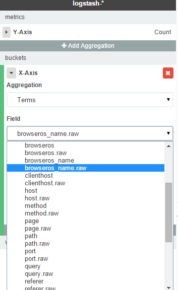
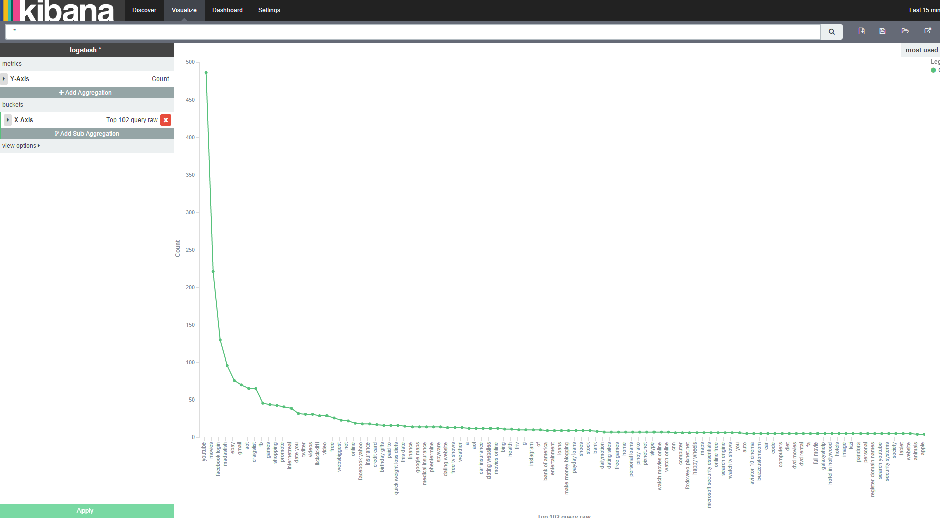 The graph shows an interesting phenomenon often seen where natural language is used.
The distribution of search queries normally follow something similar to Zipf's law, or the 80/20 rule, where 20% of the queries account for 80% of traffic.
The graph shows an interesting phenomenon often seen where natural language is used.
The distribution of search queries normally follow something similar to Zipf's law, or the 80/20 rule, where 20% of the queries account for 80% of traffic.
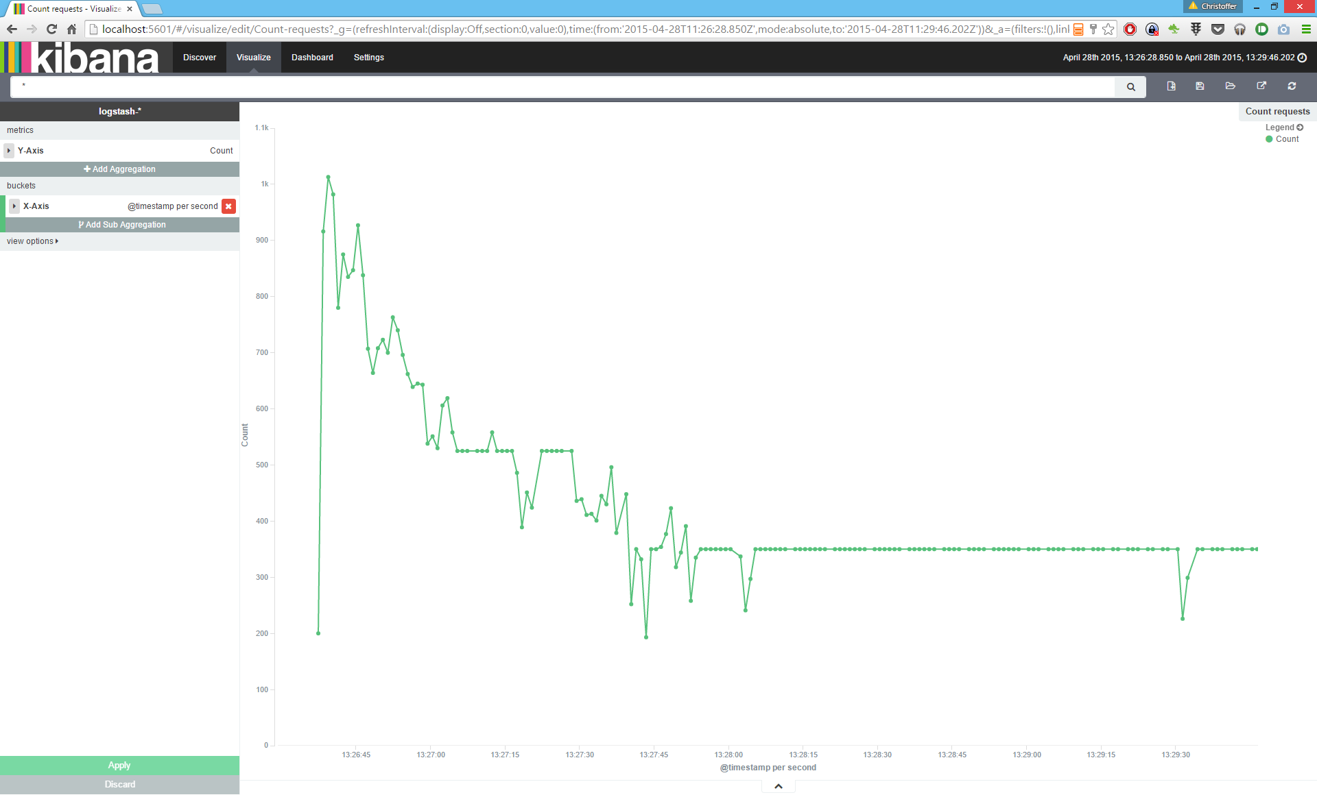
To create a graph showing the number of requests per time-slot, enter the Visualize panel, and press the little button to create a new visualization. Select "Line chart" as type of visualization, and "from a new search". Press the "Add aggregation" button, and select Aggregation type "Date histogram", and the field @timestamp. Press Apply at the bottom. If you have data (in the applied date range), you should see a graph similar to this one.
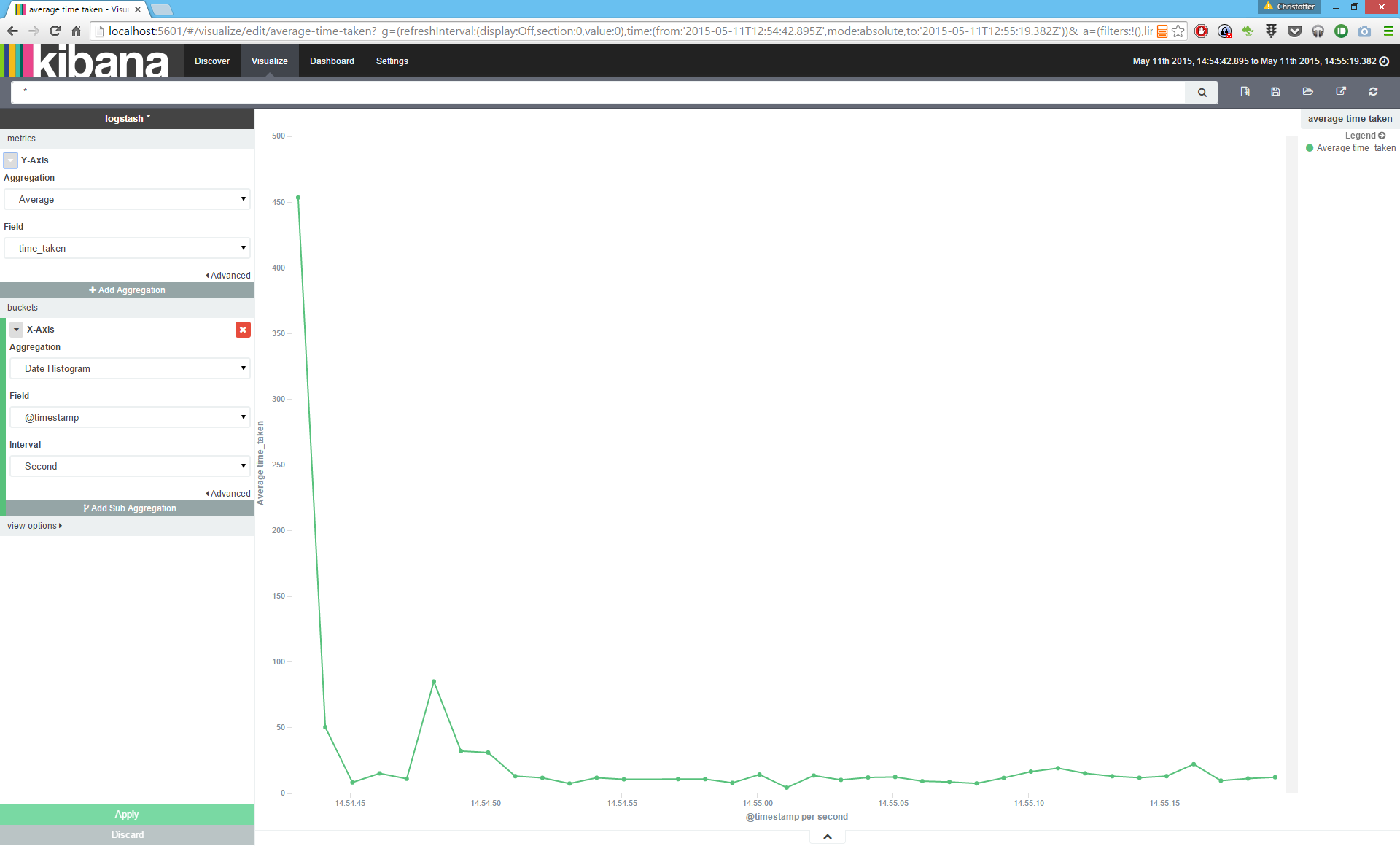
If you looked closely at the Logstash configuration, you will find that it contains a section where a field "time_taken" is converted into integer. By default, Logstash will output all fields as of type string. To work properly with numeric ranges, like the Histogram aggregation, we have to be explicit about making sure the field is of a numeric type.
Again, start a new visualization, of type "Line Chart", "from a new search". Now we are going to modify the Y-Axis, setting the type of Aggregation to Average, and using the field "time_taken" as input. For X-Axis we will use the Date histogram and the @timestamp field. Now you should see a graph displaying how the average response times varies over time.
This has been a short guide to how you can get an overview on user engagement and application performance. The ELK-stack offers a flexible toolset for analyzing and visualizing data, these steps are just scratching the surface. Hopefully, this will be enough to set you off into your own journey into the realm of the ELK-stack.
If you feel like learning more, here are some useful links:
And last - to be able to use Kibana properly, it really helps to know how aggregations work: